The Value of Dynamic Withdrawal Rules

We have written in the past about the value of tax management strategies and mentioned that Vanguard, in their Advisor’s Alpha research paper, estimated the value of all tax management strategies combined to be as high as 1.85%.  In their “Alpha, Beta, and Now… Gamma” research paper, Morningstar found that applying a dynamic withdrawal strategy can add more value than all of the tax strategies combined.  Applying a dynamic, or rules-based, approach to portfolio withdrawals sounds complicated, but the concept is simple.  In exchange for being willing to reduce spending (or at least the amount you withdraw from your portfolio) during times of poor market returns, you can start with a higher initial withdrawal rate and even increase your level of spending if investment markets continue to perform well.  The power of this strategy is derived from its management of sequence of returns risk.  Sequence of returns risk is arguably the greatest risk a retiree can face, especially for those funding a material portion of their retirement from an investment portfolio.    

Value Is Driven By Sequence of Returns Risk Management

Sequence of returns risk is generally most acute during the ten years leading up to retirement and the ten years after retiring when the portfolio’s value is likely its largest.  Sequence-of-returns risk is the risk that a series of poor returns can have an exponentially negative effect during this time frame.  Average returns can be misleading as it’s the sequence of the returns that really matter during this period of time, often referred to as the “retirement red zone.”  

As an example, assume you have two retirees, A and B. Both retirees start with $1,000,000 investment portfolios, take $50,000 annual withdrawals, and earn the same average annual return on their investment portfolios of 4.0%. The only difference is in the ordering of the hypothetical annual returns. Retiree A starts his retirement when he is blessed with a series of positive market returns followed by a series of negative returns later. Retiree B starts his retirement at the beginning of a market downturn and suffers a series of negative market returns right away, followed by positive returns later. [Note - the returns are the exact same returns, just in opposite order] 

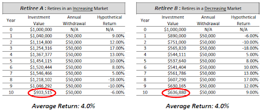
Retiree B ends up with almost $300,000, or 32%, less than Retiree A even though they had the same average return of 4.0% over the 10-year period. This example illustrates the unfortunate power of sequence-of-returns risk. The randomness of market returns matters a great deal during this retirement red zone because portfolios are large, and a given percentage change has a more significant impact on absolute wealth.

Sequence of Returns Risk Creates A Wide Possibility of Outcomes

The level of sustainable withdrawal rate from an investment portfolio is heavily influenced by what happens during this retirement red zone. These investment market-driven outcomes are unpredictable. Sequence of returns risk widens the distribution of possible outcomes in retirement.  This is why the inside of a Monte Carlo analysis, or in this example, a historical simulation analysis looks like this:

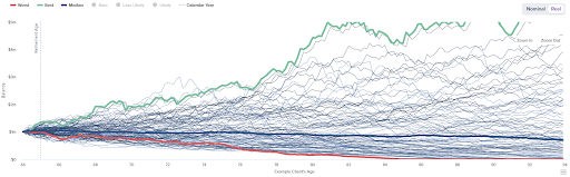
This hypothetical retiree’s worst-case observation, indicated by the red line, represents a retiree that would have retired starting in October 1905.  If this hypothetical retiree were to experience the same path of returns as someone starting retirement in October 1905, he would run out of money at age 83 years and 10 months.   The best-case observation indicated by the green line represents a retiree that would have retired starting in March 1982.  If this hypothetical retiree were to experience the same path of returns as someone starting retirement in March of 1982, he would pass having $4.18 million (in real dollars, accounting for inflation, the amount would be even more) left at age 94.  There are considerable disparities in these observations, but unfortunately, you cannot know your particular path in advance.  It is likely to be somewhere in between these observations.    

How can you be conservative if your path ends up not being as favorable but still allow yourself to participate in the upside if your path ends up being more favorable?  This is where dynamic withdrawal rules come into play.

Allowing yourself a little flexibility in your spending plan, the application of dynamic withdrawal rules can materially improve the amount you can withdrawal over your lifetime while actually taking less risk at the same time.  See a case study example in our Insight entitled “Dynamic Withdrawal Rules – Higher Withdrawals With Less Risk” for more.

What About the 4% Rule?

The “4% Rule” was born from William Bengen’s 1994 Journal of Financial Planning study “Determining Withdrawal Rates Using Historical Data.” The point of Bengen’s study was not to find what an optimal withdrawal rate would be for a retiree but rather what would have been the highest sustainable initial withdrawal rate, with inflation adjustments a retiree could have taken assuming a 50% stock (S&P 500) and 50% bond (intermediate-term government bonds) portfolio over thirty rolling thirty-year periods starting in 1926.  Bengen found the worst-case scenario occurred in the thirty-year period starting in 1966, where this hypothetical retiree would have only been able to take a 4.15% initial withdrawal rate.  

This is where the “4% rule” came from to Bengen’s chagrin.  It ignores the other 29 periods where this hypothetical retiree could have taken over 8% in the periods starting in the early 1980s and somewhere between 4% and 8% in all other periods.  Following the “4% rule” in all periods, but the one starting in 1966, would have led to a lot of money remaining on the table upon passing beyond what was planned.  That is money that could have been used to maximize happiness and contentment while living.  The “4% rule” presumes that retirees cannot make adjustments, which is just not true for most retirees.  

Dynamic Spending Rules Are Highly Customizable

The level and degree to which a retiree can make adjustments will differ given each retiree’s unique situation, but most times, there is at least a little room for adjustments.  Integrating dynamic spending rules into your retirement plan can add a great deal of potential value, whether in terms of a higher initial withdrawal rate, greater portfolio longevity, or leaving a greater legacy.  

The mainstream financial planning software products most financial advisors use cannot model the effects of dynamic spending rules. Still, there are a couple of specialist software solutions available that retirement specialists may utilize.  At Thrive Retirement Specialists, we happen to use one such solution as part of our retirement planning process.  If you would like to see how the application of  dynamic withdrawal rules can help make your retirement situation better, please contact us and we can help you model some scenarios.

CONTACT